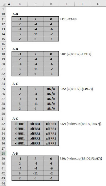
Function xlMSUB(M1, M2)
Dim rslt()
Dim i, j
Dim rws1,
rws2, cls1, cls2
rws1 =
M1.Rows.Count
cls1 =
M1.Columns.Count
rws2 =
M2.Rows.Count
cls2 =
M2.Columns.Count
ReDim
rslt(1 To rws1, 1 To cls1)
If (rws1
<> rws2) Or (cls1 <> cls2) Then
xlMSUB
= "xlERR1"
Else
For i
= 1 To rws1
For j = 1 To cls1
rslt(i, j) = M1(i, j) - M2(i, j)
Next j
Next i
xlMSUB
= rslt
End If
End Function
|
Friday, August 19, 2016
xlMatrix series: Subtracting 2 matrixes
Report any errors to afstblogs@gmail.com
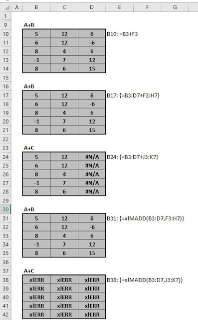
xlMatrix series: xlMADD - summing 2 matrixes
Report any errors to afstblogs@gmail.com
Function xlMADD(M1, M2)
Dim rslt()
Dim i, j
Dim rws1,
rws2, cls1, cls2
rws1 =
M1.Rows.Count
cls1 =
M1.Columns.Count
rws2 =
M2.Rows.Count
cls2 =
M2.Columns.Count
ReDim
rslt(1 To rws1, 1 To cls1)
If (rws1
<> rws2) Or (cls1 <> cls2) Then
xlMADD
= "xlERR"
Else
For i
= 1 To rws1
For j = 1 To cls1
rslt(i, j) = M1(i, j) + M2(i, j)
Next j
Next i
xlMADD
= rslt
End If
End Function
|
Tuesday, August 16, 2016
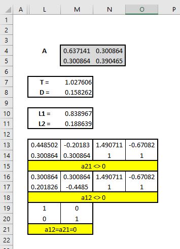
Eigenvalues and eigenvectors of 2x2 matrices
Source::
http://www.math.harvard.edu/archive/21b_fall_04/exhibits/2dmatrices/ |
M7: =M4+N5
|
M8:
=PRODUCT(M4,N5)-PRODUCT(N4,M5)
|
M10: =M7/2+SQRT(M7^2/4-M8)
|
M11: =M7/2-SQRT(M7^2/4-M8)
|
L13: =M10-N5
|
L14: =M5
|
M13: =M11-N5
|
M14: =L14
|
N13: =L13/L14
|
N14: =L14/L14
|
O13: =M13/M14
|
O14: =M14/M14
|
L16: =N4
|
L17: =M10-M4
|
M16: =N4
|
M17: =M11-M4
|
N16: =L16/L17
|
N17: =L17/L17
|
O16: =M16/M17
|
O17: =M17/M17
|
L19: 1
|
L20: 0
|
M19: 0
|
M20: 1
|
Monday, August 8, 2016
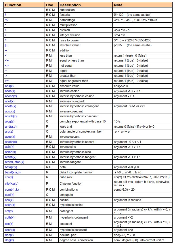
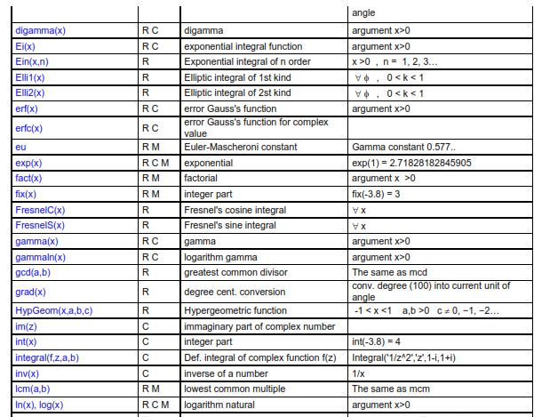
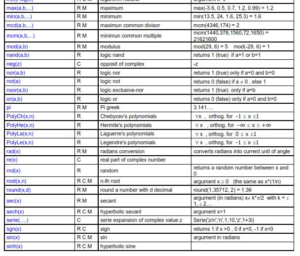
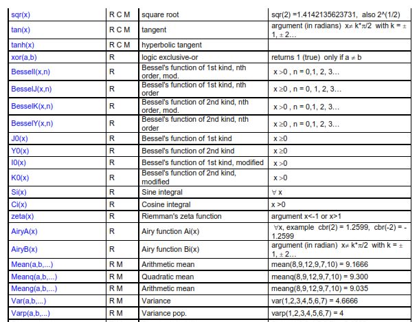
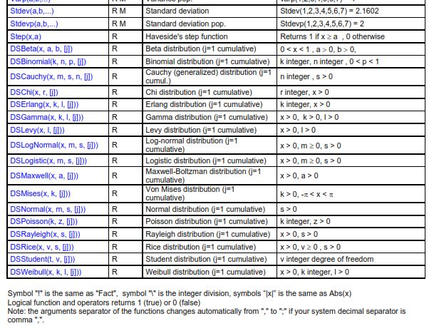
Th Xnumbers add-in: functions and special functions as presented in the Manual
All the elements presented are not warranted to be correct or free from defects.
Please report any errors found to afstblogs@gmail.com
|
About the Xnumbers add-in
The original site with the address below is no longer available.
http://digilander.libero.it/_ppricerca/index.html
Download and general informartion
http://www.thetropicalevents.com/Xnumbers60.htm |
Manual - 1
https://www.google.pt/url?sa=t&rct=j&q=&esrc=s&source=web&cd=7&cad=rja&uact=8&ved=0ahUKEwiWz_exrLHOAhXCVBQKHTlXAa0QFghSMAY&url=http%3A%2F%2Fwww.reading.ac.uk%2Fssc%2Fresource-packs%2FICRAF_2007-11-15%2Fresearch%2FResMetRes%2F5%2FHeiser%2Fnotes%2Fnoteaa.pdf&usg=AFQjCNFk20z89Gc06t5GLcIVSiqY8Lkc7w&sig2=RVy5Jd7iD3sZzeD5k1S1fA
NOTE: Many functions may seem not necessary but Xnumbers allows results with more digits than the limits of the Excel functions.
The add-in contains more functions than those listed below namely regarding special functions
NOTE: Many functions may seem not necessary but Xnumbers allows results with more digits than the limits of the Excel functions.
The add-in contains more functions than those listed below namely regarding special functions
Labels:
add-ins,
Excel,
higher precision,
Special functions,
VBA
Wednesday, August 3, 2016
Probability ellipses: *the origins (Galton 1886)
From
ANTHROPOLOGICAL MISCELLANEA
REGRESSION towards MEDIOCRITY in HEREDITARY STATURE
By FRANCIS GALTON, F.R.S. &C.
[WITH PLATES IX AND X.]
[Journal of the Anthropological Institute 15 (1886), 246–263.]
https://www.york.ac.uk/depts/maths/histstat/galton_reg.pdf
It is deduced from a large sheet on which I entered every
child's height, opposite to its mid-parental height, and in every case
each was entered to the nearest tenth of an inch. Then I counted
the number of entries in each square inch, and copied them out
as they appear in the table. The meaning of the table is best
understood by examples. Thus, out of a total of 928 children who
were born to the 205 mid- parents on my list, there were 18 of the
height of 69·2 inches (counting to the nearest inch), who were
born to mid-parents of the height of 70·5 inches (also counting to
the nearest inch). So again there were 25 children of 70·2 inches
born to mid-parents of 69·5 inches. I found it hard at first to
catch the full significance of the entries in the table, which had
curious relations that were very interesting to investigate. They
came out distinctly when I" smoothed" the entries by writing at
each intersection of a horizontal column with a vertical one, the
sum of the entries in the four adjacent squares, and using these to
work upon. I then noticed (see Plate X) that lines drawn through
entries of the same value formed a series of concentric and similar
ellipses. Their common centre lay at the intersection of the
vertical and horizontal lines, that corresponded to 68!- inches.
Their axes were similarly inclined. The points where each
ellipse in succession was touched by a horizontal tangent, lay in a
straight line inclined to the vertical in the ratio of 2/3; those where
they were touched by a vertical tangent lay in a straight line
inclined to the horizontal in the ration of 1/3. These ratios confirm
the values of average regression already obtained by a different
method, of 1/3 from mid-parent to offspring, and of 2/3 from offspring
to mid-parent, because it will be obvious on studying Plate X that
the point where each horizontal line in succession is touched by
an ellipse, the greatest value in that line must occur at the point
of contact. The same is true in respect to the vertical lines.
These and other relations were evidently a subject for mathe-
matical analysis and verification. They were all clearly dependent
on three elementary data, supposing the law of frequency of error
to be applicable throughout; these data being ( 1) the measure of
racial variability, whence that of the mid-parentages may be inferred
as has already been explained, (2) that of co-family variability
(counting the offspring of like mid-parentages as members of the
same co-family), and (3) the average ratio of regression. I noted
these values, and phrased the problem in abstract terms such as a
competent mathematician could deal with, disentangled from all
reference to heredity, and in that shape submitted it to Mr. J.
Hamilton Dickson, of St. Peter's College, Cambridge. I asked
him kindly to investigate for me the surface of frequency of error
that would result from these three data, and the various particulars
of its sections, one of which would form the ellipses to which I
have alluded.
Tuesday, July 26, 2016
Legendre polynomial (Legendre function of the first kind)
All the elements presented are not warranted to be correct or free from defects.
Please report any errors found to afstblogs@gmail.com
|
D3:
=IF(ISEVEN(B3),(-1)^(B3/2)*FACTDOUBLE(B3-1)/FACTDOUBLE(B3),0)
|
||||
D4: =xlLegendrePn(B3,B4)
|
Leave cell I4 blank
Ranges I5:K5 and N5:P5 are merged
I6: =IF(H6=0,1,IF(H6=1,$I$2,(2*H6-1)/H6*$I$2*I5-(H6-1)/H6*I4))
J6: =xlLegendrePn(H6,$I$2)
K6: =Poly_Legendre($I$2,H6)
M6: =H6
N6: =(-1)^M6*I6
O6: =xlLegendrePn(M6,-$I$2)
P6: =Poly_Legendre(-$I$2,M6)
MyExcelRoutines
This function returns only the value of the polynomial. The computation of the first derivative will be the object of a separate function.
Function xlLegendrePn(n, x)
Dim i
Dim P0, P1, Pn, Pn_1, Pn_2
P0 = 1: P1 = x
Pn_1 = P1: Pn_2 = P0
If (n <> Int(n) Or n < 0) Then
xlLegendrePn = "** n **"
ElseIf n = 0 Then
xlLegendrePn = 1
ElseIf n = 1 Then
xlLegendrePn = x
ElseIf x = 1 Then
xlLegendrePn = 1
ElseIf x = -1 Then
xlLegendrePn = (-1) ^ n
Else
For i = 2 To n
Pn = (2 * i - 1) / i * x * Pn_1 _
- (i - 1) / i * Pn_2
Pn_2 = Pn_1
Pn_1 = Pn
Next i
xlLegendrePn = Pn
End If
End Function
|
Xnumbers add-in
Poly_Legendre is an array function that returns both the values of the polynomial and its first derivative calculated by the subroutine EvalLegendre.
Function Poly_Legendre(x, Optional n)
Dim Pol#, Dpol#, k&, z#
If IsMissing(n) Then k = 1 Else k = n
z = x
Call EvalLegendre(k, z, Pol, Dpol)
Poly_Legendre = PasteVector_(Array(Pol, Dpol))
End Function
|
Sub EvalLegendre(n&, x#, Pol#,
Dpol#)
' Rutina para calcular el
polinomio ortonormal de Legendre de orden n y su derivada en x
' Los polinomios de Legendre son
un caso especial de los de Jacobi con a = b = 0
' Pol valor del polinomio en x;
DPol valor de la derivada del polinomio en x
' Bibliografia: Abramowitz M et al.; "Handbook
of Mathematical Functions...",Dover
'
Press et al.; "Numerical recipies in fotran77", Cambridge U
Press
'mod. 12.4.04 VL
Dim
k&, p#(0 To 2), dp#(0 To 2)
If n = 0
Then
Pol =
1
Dpol =
0
ElseIf n =
1 Then
Pol =
x
Dpol =
1
Else
p(0) =
1
p(1) =
x
If
Abs(x - 1) < 0.1 Or Abs(x + 1) < 0.1 Then
dp(0) = 0
dp(1) = 1
For k = 1 To n - 1
p(2) = ((2 * k + 1) * x *
p(1) - k * p(0)) / (k + 1)
'Polinomio de orden k+1 en x
dp(2)
= ((2 * k + 1) * (p(1) + x * dp(1)) - k * dp(0)) / (k + 1) 'Derivata del
polinomio di ' ordine k+1 in x .VL
p(0) = p(1)
p(1) = p(2)
dp(0) = dp(1)
dp(1) = dp(2)
Next
Pol = p(2)
Dpol = dp(2)
Else
For k = 1 To n - 1
p(2) = ((2 * k + 1) * x *
p(1) - k * p(0)) / (k + 1)
' Polinomio de orden k+1 ' ' en x
p(0)
= p(1)
' (***)
p(1) = p(2)
Next
Pol = p(2)
Dpol = n * (x * p(2) - p(0)) / (x ^ 2 - 1) ' Derivada del polinomio de orden k+1
en x
End If
End If
End Sub
|
From the Tutorial -1:
Matlab
Values of Pn(x)
Polynomials
Friday, June 17, 2016
Three ways to use Excel worksheet functions in VBA
Function xlAverage01(rng)
xlAverage01 =
WorksheetFunction.Average(rng)
End Function
Function xlAverage02(rng)
With WorksheetFunction
xlAverage02 = .Average(rng)
End With
End Function
Function xlAverage03(rng)
Dim wsf As WorksheetFunction
Set wsf = WorksheetFunction
xlAverage03 = wsf.Average(rng)
End Function
|
Thursday, June 2, 2016
Mix-up about the covariance in Excel
One of the Excel mix-ups in its statistical functions that lasted longer is about the computation of the covariance.
Until recently (we think that this change was only introduced in the 2007 version) Excel provided two functions for the variance and standard deviation, one,for population and the other for sample data.
However, there was only one function for the covariance that returned the value for population data. There was (an there is) also only one function for the correlation, which is right, since the correlation values are the same for population ans sample data. This situation could lead to the erroneous conclusion that the covariance also has the same value for both cases.
The fixing of this situation was made by introducing two formulas for the computation of the covariance.
However, the procedure Covariance of the Analysis ToolPak still returns the population covariances. Additionally, it also maintains another heritage mix-up. Although the Toolpak general methodology presents fixed values in the output, that does not change automatically if data values change, in this case the diagonals of the covariance matrix contain the formula to compute the population variance. This means that changes in the data will automatically change values in the diagonal, contrary to what happens for the other elements of the matrix.
The matrix.xla add-in, presented in another message also has only one function for the covariance matrix that returns the values for population data.
Wednesday, June 1, 2016
Generating correlated normal random numbers - Part 01
This function generates five columns containing numbers (the headers are not generated by the function):
Source:
https://www.blogger.com/blogger.g?blogID=3230308801600609435#editor/target=post;postID=4988601992196925693;onPublishedMenu=posts;onClosedMenu=posts;postNum=1;src=postname
In a future message the remaining models in the source will be presented.
The code for the function xlCorrMtx is in this blog at
https://www.blogger.com/blogger.g?blogID=3230308801600609435#editor/target=post;postID=4988601992196925693;onPublishedMenu=posts;onClosedMenu=posts;postNum=1;src=postname
- Order number (i)
- Uniform random sequence (Z1)
- Uniform random sequence (Z2)
- First combination of Z1 and Z2 >>> Z3
- Second combination of Z2 and Z1 >>> Z4
The pairs (Z1,Z3) and (Z2,Z4) simulate a sample extracted from populations in which the pairs have a chosen value for the correlation. As it happens in sampling you usually get a value for the sampling correlation that differs from the population.
The values returned can be unstandardized specifying for each case the mean and standard deviation.
If you are not satisfied with the outcome, recalculate the spreadsheet. As the random values are generated by VBA code they are not volatile as it happens when you input the Excel built-in RAND function in a spreadsheet cell.
See more about volatility in the follow link in a post entitled Handle Volatile Functions like they are dynamite:
The inputs are:
- Number of lines in the sequences (k)
- Value of population correlation
https://www.blogger.com/blogger.g?blogID=3230308801600609435#editor/target=post;postID=4988601992196925693;onPublishedMenu=posts;onClosedMenu=posts;postNum=1;src=postname
B6:E9 | {=xlCorrMtx(B12:E41)} |
A12:E41 | {=xlRndNormal(C3,E3)} |
H6:K9 | {=xlCorrMtx(H12:K41)} |
H12 | =H$3+B12*H$4 |
Function xlRndNormal(k As Integer, corr)
With WorksheetFunction Dim i As Integer Dim rslt() ReDim rslt(1 To k, 1 To 5) For i = 1 To k rslt(i, 1) = i Next i For i = 1 To k rslt(i, 2) = .Norm_S_Inv(Rnd) Next i For i = 1 To k rslt(i, 3) = .Norm_S_Inv(Rnd) Next i For i = 1 To k rslt(i, 4) = corr * rslt(i, 2) + Sqr(1 - corr ^ 2) * rslt(i, 3) Next i For i = 1 To k rslt(i, 5) = corr * rslt(i, 3) + Sqr(1 - corr ^ 2) * rslt(i, 2) Next i xlRndNormal = rslt End With End Function |
The code for the function xlCorrMtx is in this blog at
https://www.blogger.com/blogger.g?blogID=3230308801600609435#editor/target=post;postID=4988601992196925693;onPublishedMenu=posts;onClosedMenu=posts;postNum=1;src=postname
Sample covariance matrix
Function xlCovSMtx(rng As Range)
Dim i, j
Dim nCls As Integer
Dim mtx()
With WorksheetFunction
nCls =
rng.Columns.Count
'MsgBox nCls
ReDim mtx(1 To nCls, 1
To nCls)
For i = 1 To nCls
For j = 1 To nCls
mtx(i, j) =
.Covariance_S(rng.Columns(i), rng.Columns(j))
Next j
Next i
xlCovSMtx = mtx
End With
End Function
Function xlCovSMtx_U(rng As Range)
Dim i, j
Dim nCls As Integer
Dim mtx()
With WorksheetFunction
nCls =
rng.Columns.Count
'MsgBox nCls
ReDim mtx(1 To nCls, 1
To nCls)
For i = 1 To nCls
For j = 1 To nCls
If i <= j
Then
mtx(i, j) =
.Covariance_S(rng.Columns(i), rng.Columns(j))
Else
mtx(i, j) =
0
End If
Next j
Next i
xlCovSMtx_U = mtx
End With
End Function
Function xlCovSMtx_L(rng As Range)
Dim i, j
Dim nCls As Integer
Dim mtx()
With WorksheetFunction
nCls = rng.Columns.Count
'MsgBox nCls
ReDim mtx(1 To nCls, 1
To nCls)
For i = 1 To nCls
For j = 1 To nCls
If i >= j
Then
mtx(i, j) =
.Covariance_S(rng.Columns(i), rng.Columns(j))
Else
mtx(i, j) =
0
End If
Next j
Next i
xlCovSMtx_L = mtx
End With
End Function
|
Sunday, May 29, 2016
Correlation matrix
Dim i, j
Dim nCls As Integer
Dim mtx()
With WorksheetFunction
nCls = rng.Columns.Count
'MsgBox nCls
ReDim mtx(1 To nCls, 1 To
nCls)
For i = 1 To nCls
For j = 1 To nCls
mtx(i, j) =
.Correl(rng.Columns(i), rng.Columns(j))
Next j
Next i
xlCorrMtx = mtx
End With
End Function
Function xlCorrMtx_U(rng As Range)
Dim i, j
Dim nCls As Integer
Dim mtx()
With WorksheetFunction
nCls = rng.Columns.Count
'MsgBox nCls
ReDim mtx(1 To nCls, 1 To
nCls)
For i = 1 To nCls
For j = 1 To nCls
If i <= j Then
mtx(i, j) =
.Correl(rng.Columns(i), rng.Columns(j))
Else
mtx(i, j) = 0
End If
Next j
Next i
xlCorrMtx_U = mtx
End With
End Function
Function xlCorrMtx_L(rng As Range)
Dim i, j
Dim nCls As Integer
Dim mtx()
With WorksheetFunction
nCls = rng.Columns.Count
'MsgBox nCls
ReDim mtx(1 To nCls, 1 To
nCls)
For i = 1 To nCls
For j = 1 To nCls
If i >= j Then
mtx(i, j) =
.Correl(rng.Columns(i), rng.Columns(j))
Else
mtx(i, j) = 0
End If
Next j
Next i
xlCorrMtx_L = mtx
End With
End Function
|
Subscribe to:
Posts (Atom)